Adding ML to the "P"

Multilayer Perceptron

Early in the section for perceptron, we saw it as being an algorithm (or as can be said, an analog machine) that is basically a linear classifier. Now, in the MLP, the layer in itself is a linear function, but from one layer to another, nonlinearity can be introduced by use of activation functions.
So what are activation functions? - they are just mathematical functions that are introduced at the end of units to introduce non-linear complexities to the model. sgn is not non-linear because it is not-differentiable, hence why we couldn't have computed the gradients the Pytorch way while implementing the perceptron.

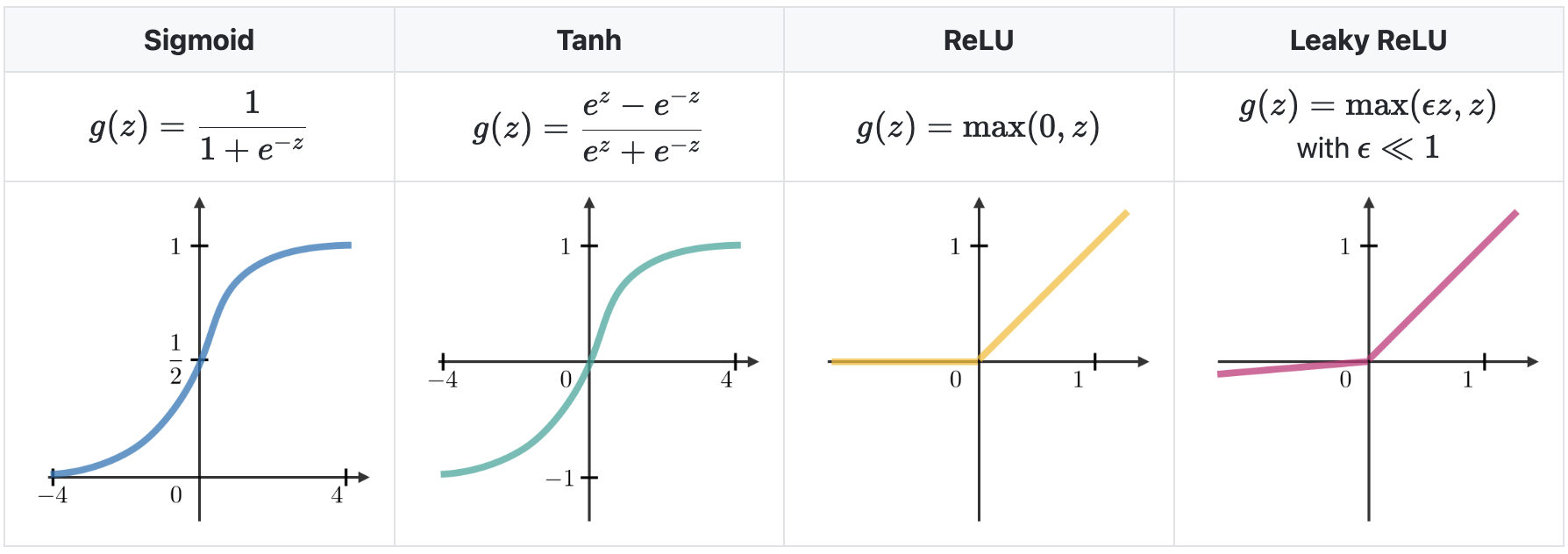
courtesy of Stanford deep learning cheatsheet

Demystifying MLP

So how does a single layer perceptron look like? Let's understand this programmatically by creating one composed of 4 perceptrons.

The approach to implementing this is by first using naive for loop to stack each perceptron side by side then it is efficiently implemented using a matrix block that specifies the weights and the biases.

But first, let's create a Linear layer, PyTorch's implementation of perceptrons stacked side by side, or as the cheat sheet above visualizess it, one perceptron on top of another the 4 blue nodes on top each other.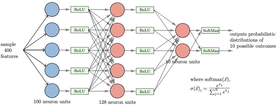

torch.manual_seed(42)
# initialize 3 samples of 7 features each
samples = torch.randn(3, 7)
# create layer of 4 perceptrons considering 7 features
layer = nn.Linear(7, 4)
out = layer(samples)
# your values for out might be different from mine
# that's fine, know they will be consistent when you
# rerun the code
print(out)

            tensor([[ 0.6222,  0.1250, -0.6566,  0.5412],
        [ 0.2936,  0.7253, -0.9345,  0.4647],
        [-0.5043,  0.5410, -0.5203, -0.3301]], grad_fn=<AddmmBackward0>)
          

Let's start with the perceptron, but without the activation function (without the sgn function used in the previous section or a differentiable function like tanh) since PyTorch's version doesn't have an activation function within.

class OnePerceptron:
    def __init__(self, shape_x):
        super().__init__()
        self.w = torch.randn(shape_x)
        self.b = torch.randn(1)

    def __call__(self, x):
        out = torch.dot(x, self.w) + self.b
        return out

Now onto stacking n number of perceptrons side by side, the exact number to be specified during instantiation.

class ManyPerceptrons:
    def __init__(self, feature_shape, units=1):
        self.perceptrons = []
        # naive implementation
        # stacking perceptrons side by side 
        # in a single layer
        for _ in range(units):
            self.perceptrons.append(OnePerceptron(feature_shape))
        print(f"{len(self.perceptrons)} perceptrons ==> shape {feature_shape}")

Knowing that the input is passed to each node, then the perceptron computes the result, let's implement the __call__ magic method to do this.

# ...
# continuing on within ManyPerceptrons class
def __call__(self, x):
    out_all_perceptrons = []
    for p in self.perceptrons:
        out = p(x)
        out_all_perceptrons.append(float("{:.4f}".format(out.item())))
    return out_all_perceptrons

Note: the formatting done above is just to reduce floating point precision to 4 dp to reduce verbosity.
Now, initializing my single-layer, 4 perceptrons stacked side by side. Or any number of perceptrons you wish to have.

torch.manual_seed(42) # if using jupyter notebook, this should be in same cell
slPerceptron = ManyPerceptrons(samples[0].shape, 4)
for sample in samples:
    out_each = slPerceptron(sample)
    print(out_each)

            4 perceptrons ==> shape torch.Size([7])
[0.7342, -0.838, 6.8438, 2.8546]
[-0.2729, 3.1664, 3.7544, 0.3837]
[-2.8693, 3.1136, 2.5533, 0.2767]
          

Now let's do something interesting, let's transfer weights from PyTorch's Linear layer to the naive implementation. If the two are the same architecture, then the output should actually be the same.

# transfer weights and biases from pytorch implementation of single Layer Perceptron (Linear)
# to see that we've actually built the same thing
weights, biases = layer.parameters()

for i, (
    weights_in_each_perceptron, 
    bias_in_each_perceptron
) in enumerate(zip(weights, biases)):
    slPerceptron.perceptrons[i].w[:] = weights_in_each_perceptron
    slPerceptron.perceptrons[i].b[:] = bias_in_each_perceptron
    # [:] ensures we maintain the same underlying object,
    # only modifying the values

Computing the outputs

for sample in samples:
    out_naive = slPerceptron(sample)
    print(out_naive)

            [0.6222, 0.125, -0.6566, 0.5412]
[0.2936, 0.7253, -0.9345, 0.4647]
[-0.5043, 0.541, -0.5203, -0.3301]
#
###########################
##  same result, nice!!! 
###########################
          

Now let's actually utilize the compactness of matrices to implement an efficient version of the 4 perceptrons stacked side by side (what I call the single layer perceptron).

class ManyPerceptronsEfficient:
    def __init__(self, shape_x, units=1):
        super().__init__()
        self.w = torch.randn(units, shape_x, requires_grad=False)
        self.b = torch.randn(1, units, requires_grad=False)

    def __call__(self, x):
        out = torch.matmul(x, self.w.T) + self.b
        return out

Again, copying weights and biases from the Linear layer!

pEfficient = ManyPerceptronsEfficient(samples[0].shape[0], 4)
# again, copying weights from the pytorch instance
pEfficient.w[:] = weights
pEfficient.b[:] = biases
for sample in samples:
    out_each = pEfficient(sample.unsqueeze(0))
    print(out_each)

            tensor([[ 0.6222,  0.1250, -0.6566,  0.5412]], grad_fn=<AddBackward0>)
tensor([[ 0.2936,  0.7253, -0.9345,  0.4647]], grad_fn=<AddBackward0>)
tensor([[-0.5043,  0.5410, -0.5203, -0.3301]], grad_fn=<AddBackward0>)
          

out_all = pEfficient(samples)
print(out_all)

            tensor([[ 0.6222,  0.1250, -0.6566,  0.5412],
        [ 0.2936,  0.7253, -0.9345,  0.4647],
        [-0.5043,  0.5410, -0.5203, -0.3301]], grad_fn=<AddBackward0>)
#
###########################
##  again same result!!! 
###########################
          

The class created above, can be rewritten as a base PyTorch class using the torch.nn.Module, the base class for PyTorch models, as seen below

import torch.nn as nn

class ManyPerceptronsPT(nn.Module):
    def __init__(self, shape_x, units=1, batch_size=1):
        super().__init__()
        self.batch_size = batch_size
        self.w = torch.randn(units, shape_x, requires_grad=False)
        self.b = torch.randn(1, units, requires_grad=False)

    def forward(self, x):
        out = torch.matmul(x, self.w.T) + self.b
        return out

All this was for the understanding of Linear layer, for which the in-built PyTorch module described at the beginning is recommended for use.
Multiple layers of the perceptrons stacked side by side is what is now known as "Multilayer Perceptron", and is as below in code implementation

mlp = nn.Sequential(
    nn.Linear(in_features = 400, out_features = 100),
    nn.ReLU(),
    nn.Linear(in_features = 100, out_features = 128),
    nn.ReLU(),
    nn.Linear(in_features = 128, out_features = 10),
    nn.Softmax(dim=1)
)
print(mlp(torch.randn(1, 400)))

            tensor([[0.1164, 0.0934, 0.1123, 0.1057, 0.0991, 0.0944, 0.0966, 0.0794, 0.1028,
        0.0999]], grad_fn=<SoftmaxBackward0>)
          