The foundations for residual learning
As the semiconductor industry advanced in the many-thread trajectory which focused more on the execution through-put of parallel applications, hardware was no longer a limiting factor in training deeper neural networks (networks with so many layers), gradients were.
The AI research community, driven by the significance of depth, wanted to answer the question: Is learning better networks as easy as stacking more layers?. However, as the layers were more, an obstacle arose, the notorious problem of vanishing or exploding gradients.
During backpropagation of deep networks, gradients of loss with respect to the weights for each neuron-processing node are computed. The gradients then, with a given optimizer, updates the weights of the neuron-processing nodes. Since these gradients are successively calculated (back-propagated) through the chain rule from the output layer to the input layer, where each layer contributes its own gradient to the previous layer’s gradient, they can diminish exponentially with each additional layer, resulting in vanishing gradients.
The paper,,Deep Residual Learning for Image Recognition, then decided to focus on a framework to ease the training of networks significantly deeper than those used previously.
And I quote from the paper,
There exists a solution by construction to the deeper model: the added layers are identity mapping, and the other layers are copied from the learned shallower model. The existence of this constructed solution indicates that a deeper model should produce no higher training error than its shallower counterpart.
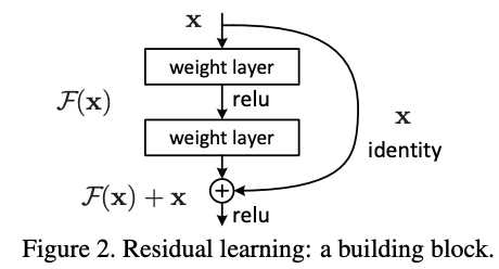
The figure above therefore entails the structure of a residual block, having a tap from shallower layers, skipping over two layers, then merging with the outputs. From the paper, the weight layers in the residual block are convolutional layers. But what is a convolution layer, and what is convolution? There's so much to explore, yet so few still understood. For that reason, let's pause this and go back in time to when convolution first had its meaning.
Convolution?
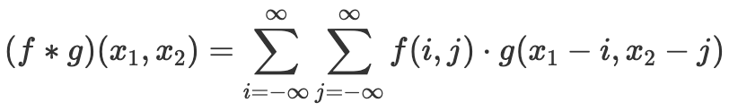
Being the most important building block of a Convolution Neural Network, a convolution layer implements a convolution,
A convolution is a mathematical operation that slides one function over another and measures the integral of their pointwise multiplication. For discrete points, the integral becomes the sum. Convolutional layers actually use cross-correlations, which are very similar to convolutions except that in convolution, one of the functions is mirrored.
A convolution is a mathematical operation that slides one function over another and measures the integral of their pointwise multiplication. For discrete points, the integral becomes the sum. Convolutional layers actually use cross-correlations, which are very similar to convolutions except that in convolution, one of the functions is mirrored.
For more explanation of the above, you can have a fun read at
A guide to convolution arithmetic for deep learning
A guide to convolution arithmetic for deep learning
Let's limit ourselves to 2D convolution, and hence 2D convolutional layer.
Imagine an input feature map, like a single channel in an RGB image, size 28 by 28, and a kernel, of some size 3 by 3. This kernel has some values in its matrix, can be random, can be defined for let's say edge detection or denoising. The kernel is then applied to a patch of the input feature map which is 3 by 3 (the elementwise multiplication of elements of kernel and the patch) then summed to a single value. The kernel then slides to another patch in the image and then computes the same until it moves over the whole image. Simply put, location shifted versions of the kernel is applied across the entire input feature map.
Imagine an input feature map, like a single channel in an RGB image, size 28 by 28, and a kernel, of some size 3 by 3. This kernel has some values in its matrix, can be random, can be defined for let's say edge detection or denoising. The kernel is then applied to a patch of the input feature map which is 3 by 3 (the elementwise multiplication of elements of kernel and the patch) then summed to a single value. The kernel then slides to another patch in the image and then computes the same until it moves over the whole image. Simply put, location shifted versions of the kernel is applied across the entire input feature map.
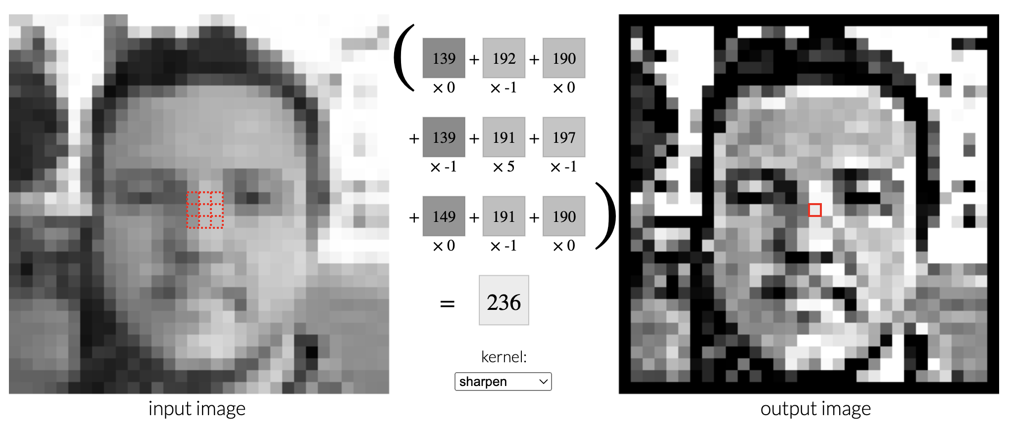
courtesy of,Image Kernels
For the given patch of image above, the implementation is as below:
For the given patch of image above, the implementation is as below:
            tensor([[ 0., -1.,  0.],
        [-1.,  5., -1.],
        [ 0., -1.,  0.]])
tensor([[139, 192, 190],
        [139, 191, 197],
        [149, 191, 190]])
tensor(236.)
A filter is a depthwise stack of kernels. As much as some articles use kernels and filters interchangeably, a filter can be clearly known as defined above. Hence, for a image of 3 channels, the filter will also have 3 kernels stacked depthwise, such that the discrete convolution sums the result of each channel to have a scalar output. Similarly, an n-channel feature map will have a n-channel filter.
single-channel convolution
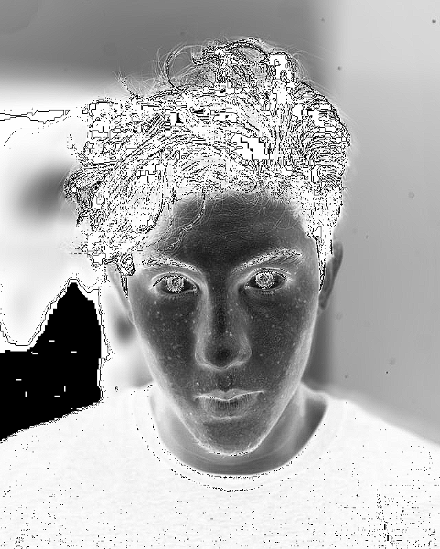
Now that we have implemented multiplication sum on the patch, let's convolve a sharpen kernel with the entire image in a single channel.
Photo by ~Erik Lucateroon ~Unsplash
First things first, let's load the image
Photo by ~Erik Lucateroon ~Unsplash
First things first, let's load the image

So, the code above does compute the convolution across the entire single-channel image, resulting in an output that is generally defined by
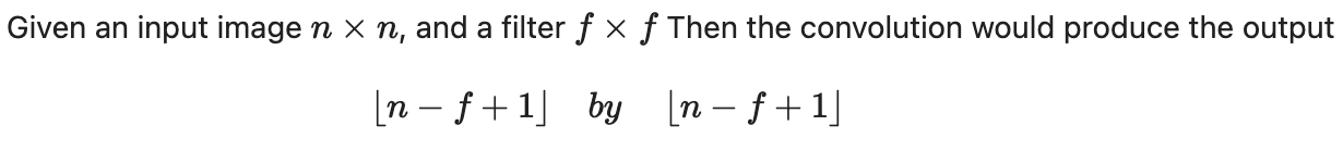
Hence why the output for the convolution is defined by the dimensions H-SIZE+1 and W-SIZE+1. The kernel needs to be bound within the image limits, hence why the range is defined as so, using offset to control the kernel as it slides over the image during the convolution operation.
Implementing the convolution in PyTorch and asserting that the two are actually the same, we have
Implementing the convolution in PyTorch and asserting that the two are actually the same, we have
True
Next, while still exploring convolution, let's see operations applied with convolution such as strides and padding, strides being the number of steps taken as the kernel moves across the feature map, in the previous code example it was 1, and padding being the number of zeros around the image.
strides control the output spatial dimension while padding ensures the information around the borders of a feature map are not lost.
More in-depth on convolution,,From Convolution to Neural Network
strides control the output spatial dimension while padding ensures the information around the borders of a feature map are not lost.
More in-depth on convolution,,From Convolution to Neural Network