Playing with Grads

Once upon an apple...

at a time when Isaac Newton lived

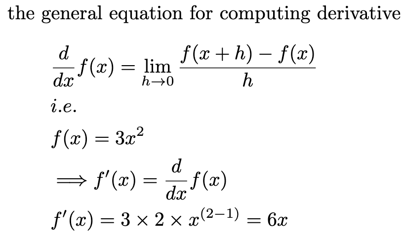
There existed the calculus ofgradients, a fancy word to say derivatives, or the rate of change of a function.

implementing the gradient above programmatically, pytorch requires inputs to a function be a Tensor with grad set to true, as seen in the initialization below, enabling the creation of a graph for tracking the operations and computing the gradients in the backward pass. This is the most fundamental concept in training neural networks, forward propagation and backward pass.\

import torch 

# derivative evalauted at x = 3.0
def f(x):
    return 3 * x ** 2
    
def derivative(f, a, h = 0.001):
    return (f(a + h) - f(a)) / h

x = torch.tensor(3.0, requires_grad = True)
y = f(x)
y.backward()

basic_derivative = derivative(f, 3)
torch_derivative = x.grad

print(f"naive diff : {basic_derivative:.1f}")
# naive diff : 18.0
print(f"torch diff : {torch_derivative}")
# torch diff : 18.0

Let's now understand better from a chain of operations, but before we continue further...

note that torch.Tensor returns a Torch.FloatTensor while torch.tensor infers the dtype automatically. It can also be noted that torch.Tensor does not have arguments like requires_grad, dtype, so torch.tensor is used in this case. In general, torch.tensor is recommended.

a = torch.Tensor(4)
b = torch.tensor(4)

c = np.arange(0, 1, 0.2)
d = torch.Tensor(c)
e = torch.tensor(c)

g = torch.Tensor([1, 2, 4])
h = torch.tensor([1, 3, 5]).to(torch.float32).to("mps")

i = torch.tensor([[3, 0],[4, 5]], dtype=torch.float32)
j = i.matmul(i) # element-wise multiplication is ===> i * i

print(f"{a=}\n{b=}\n{d=}\n{e=}\n{g=}\n{h=}\n{i=}\n{j=}")

            [Python]$ python3 playingWithGrads.py 
a=tensor([0., 0., 0., 0.])
b=tensor(4)
d=tensor([0.0000, 0.2000, 0.4000, 0.6000, 0.8000])
e=tensor([0.0000, 0.2000, 0.4000, 0.6000, 0.8000], dtype=torch.float64)
g=tensor([1., 2., 4.])
h=tensor([1., 3., 5.], device='mps:0')
i=tensor([[3., 0.],
        [4., 5.]])
j=tensor([[ 9.,  0.],
        [32., 25.]])
          

Also note, for requires_grad to not create an error, the data must be float data type. That is since for gradients to be defined, you need a continuous function, and float data is the way to represent continuity in such functions.
Note that the code below will give an error.

a = torch.tensor(4, requires_grad=True)

But when modified as below, it works okay.

a = torch.tensor(4, dtype=torch.float32, requires_grad=True)
# OR
a = torch.tensor(4.0, requires_grad=True)

back to our computational graph

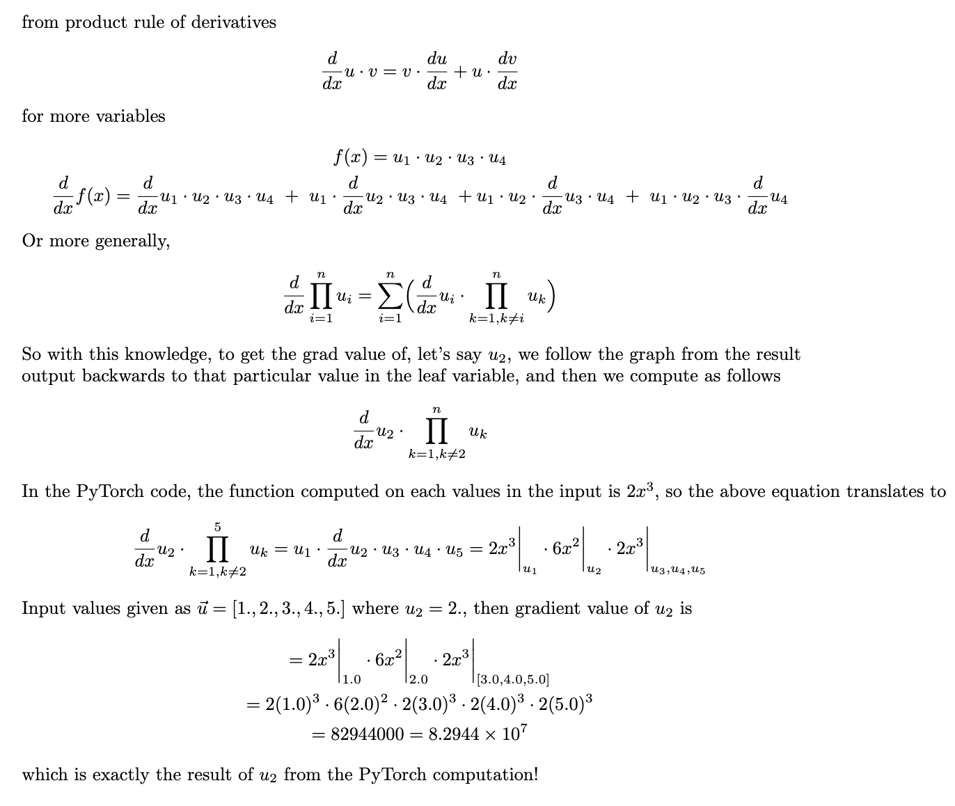
Let's continue on, learning something interesting on compounded operations on computational graphs from the sum of gradients and on the product of gradients.
Essentially, the gradient of sums is the sum of gradients, hence for the computational graph as seen below, the gradient of a particular value in the leaf variable (to be explained what it means in a bit) does not depend on any other associated variable in the leaf variable.

x = torch.tensor([1., 2., 3., 4., 5.], requires_grad=True)
y = 2 * x ** 3
# for autograd to work, the output needs to be a scalar
# so let's sum the results of y to a scalar.
z = torch.sum(y)
z.backward()
print(z)
print(x.grad)

            [Python]$ python3 playingWithGrads.py 
tensor(450., grad_fn=<SumBackward0>)
tensor([  6.,  24.,  54.,  96., 150.])
          

Let's get into a bit more fun, understand mathematically and programmatically what happens when we change the torch.sum to torch.prod and derive the result

x = torch.tensor([1., 2., 3., 4., 5.], requires_grad=True)
y = 2 * x ** 3
z = torch.prod(y)
z.backward()
print(x)
print(x.grad)

            [Python]$ python3 playingWithGrads.py 
tensor(55296000., grad_fn=<ProdBackward0>)
tensor([1.6589e+08, 8.2944e+07, 5.5296e+07, 4.1472e+07, 3.3178e+07])
          

# from the resulting simplication, the other values can be reproduced as
def grad_of_xs(xs):
    # detach is used to remove the computational graph of the variable
    # as to not mess with the gradient computation of the graph
    xs = xs.detach()
    grad_xs = torch.zeros(len(xs))
    for i, x in enumerate(xs):
        grad_xs[i] = 6 * x ** 2 * torch.prod(2 * xs[xs != x] ** 3)
        print(grad_xs[i])
    return grad_xs

grad_values = grad_of_xs(x)
print(grad_values)
assert torch.equal(grad_values, x.grad), "NOT PASSED, COMPUTATIONS NOT SAME"

            [Python]$ python3 playingWithGrads.py 
tensor(1.6589e+08)
tensor(82944000.)
tensor(55296000.)
tensor(41472000.)
tensor(33177600.)
tensor([1.6589e+08, 8.2944e+07, 5.5296e+07, 4.1472e+07, 3.3178e+07])
          

As can be seen, the computational graph is very essential and it is used in updating of weights in neural networks based on the gradients computed from the operations in the computational graph.
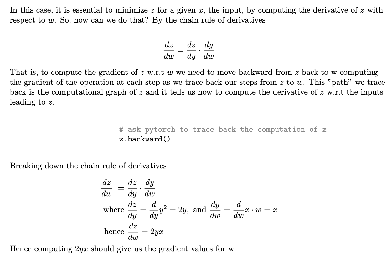
Let's understand one more of the computation graphs based on the chain rule of derivatives

torch.manual_seed(42)

x = torch.rand(4, requires_grad=True)
w = torch.rand(4, requires_grad=True)

print("x values: ")
print(x)
print("w values: ")
print(w)
y = x @ w  # inner-product of x and w
z = y ** 2
z.backward()
print("z:")
print(z)
print("w grad values:")
print(w.grad)

            x values: 
tensor([0.8823, 0.9150, 0.3829, 0.9593], requires_grad=True)
w values: 
tensor([0.3904, 0.6009, 0.2566, 0.7936], requires_grad=True)
z:
tensor(3.0761, grad_fn=<PowBackward0>)
w grad values:
tensor([3.0948, 3.2096, 1.3430, 3.3650])
          

x = x.detach()
y = y.detach()
w_manual_grad_result = 2*y*x
print(f"manual grad calculation: \n{w_manual_grad_result}")
print(f"torch grad calculation: \n{w.grad}")
assert torch.equal(w_manual_grad_result, w.grad), "results not same"

            manual grad calculation: 
tensor([3.0948, 3.2096, 1.3430, 3.3650])
torch grad calculation: 
tensor([3.0948, 3.2096, 1.3430, 3.3650])
          

Dealing with computational graphs has been interesting. For more in-depth and thorough understanding of the computational graphs, that is the construction of the graphs in PyTorch and the execution of the graphs, look into these awesome articlescomputational graphs constructedandcomputational graphs execution

before we finish

Remember us talking about leaf Tensors. This is a variable that is at the beginning of a graph. These variables are the only variables that we can acquire the gradients using .grad. For instance, in the previous computations, we cannot access the gradients of y or of z because they do not start the graph.

print("x is leaf:")
print(x.is_leaf)
print("w is leaf:")
print(w.is_leaf)
print("y is leaf:")
print(y.is_leaf)
print("z is leaf:")
print(z.is_leaf)

            x is leaf:
True
w is leaf:
True
y is leaf:
False
z is leaf:
False
          

Let us look into some variable initialization in Pytorch and see if they are characteristic of a leaf Tensor.

#############################################################
#                                                           # 
#   A leaf Variable is a variable that is at the beginning  #
#   of the graph. That means that no operation tracked by   #
#           the autograd engine created it.                 #
#  This is what you want when you optimize neural networks  # 
#       as it is usually your weights or input.             #
#                                                           # 
#############################################################
#                                                           # 
#   So to be able to give weights to the optimizer, they    #
#   should follow the definition of leaf variable above.    #
#                                                           # 
#############################################################
#
check_is_leaf = lambda x: print(f"a is leaf {x.is_leaf}")

a = torch.rand(10, requires_grad=True) 
check_is_leaf(a)
# a is a leaf variable

a = torch.rand(10, requires_grad=True).double() 
check_is_leaf(a)
# a is NOT a leaf variable as it was created by the operation 
# that cast a float tensor into a double tensor
# note that rand automatically casts the value passed to float
# hence why before the .double(), it is a float

a = torch.rand(10).requires_grad_().double()
check_is_leaf(a)
# equivalent to the formulation just above: not a leaf variable

a = torch.rand(10).double() 
check_is_leaf(a)
# not the result of an operation, is a leaf Tensor

a = torch.rand(10).double().requires_grad_() 
check_is_leaf(a)
# is a leaf variable because the requires_grad is applied
# in place after the casting operation

a = torch.rand(10, requires_grad=True, device="mps")
check_is_leaf(a)
# a requires grad, has no operation creating it: it's a leaf 
# variable as well and can be given to an optimizer

a = torch.rand(10, requires_grad=True)
a = a.to("mps")
check_is_leaf(a)
# is not a leaf Tensor, as the value was moved to the mps from 
# the cpu by the .to function, and not done in place as
# is the case with the previous function

            a is leaf True
a is leaf False
a is leaf False
a is leaf True
a is leaf True
a is leaf True
a is leaf False
          

With this look into passing input Tensor into a function to get the output foward pass, then doing a .backward() to compute the gradients of the leaf Tensor ( backpropagation ) is the very core of optimization, which we'll have fun exploring in future sections.