Pooling layers

Max Pooling

Hey, welcoming back! In this section, let's start with pooling, an operation that slides over patches of feature map just like the convolution, but instead it has no weights and its purpose is to reduce the dimensionality of feature map. It can be seen as a strided convolution with a specific constant kernel. For this reason, all the parameters we've learned such as stride, padding, are in PyTorch's implementation of the concept.
There is MaxPool2d and AvgPool2d, the first one taking the maximum of the patch in the input feature map while the second takes the average of the patch of the feature map.

def naive_pooling(feature_map, kernel_size, strides, padding, avg=False):
    feature_map = (naive_padding(feature_map, padding) 
                if padding else feature_map)
    SIZE = kernel_size
    (H, W) = feature_map.shape
    out_H = int(((H-SIZE)/strides)+1)
    out_W = int(((W-SIZE)/strides)+1)
    output_naive = torch.zeros(out_H, out_W)
    pool_fn = torch.mean if avg else torch.max
    for i in range(out_H):
        for j in range(out_W):
            r = i * strides
            c = j * strides
            patch = feature_map[r:r+SIZE, c:c+SIZE]
            value = pool_fn(patch)
            output_naive[i, j] = value
    return output_naive

From the implementation, since there difference in MaxPool2d and AvgPool2d is in the operation within the patch, this involves a one line modification to incorporate the operation needed at the time of function call. However, in the official implementation, it involves separating the two since it's easier for optimizations while handling the internals in parallel computing. Since PyTorch is to work for optimizations in different hardware accelerators, it therefore makes most sense to modularize each implementation to reduce unnecessary checks.

import torch.nn as nn
x = torch.arange(1,13).reshape(3,4).to(torch.float)

maxPool2d = nn.MaxPool2d(kernel_size=2,stride=2, padding=1)
avgPool2d = nn.AvgPool2d(kernel_size=2,stride=2, padding=1)

out_max = maxPool2d(x.view(1,1,*x.shape))
out_avg = avgPool2d(x.view(1,1,*x.shape))

out_max = out_max.squeeze(0).squeeze(0)
out_avg = out_avg .squeeze(0).squeeze(0)

out_max_2 = naive_pooling(x,2,2,1)
out_avg_2 = naive_pooling(x,2,2,1, True)

print("Pooling match: max: {} avg: {}".format(
    torch.equal(out_max, out_max_2),
    torch.equal(out_avg, out_avg_2)
))

            Pooling match: max: True avg: True
          

So, what is global average pooling? Imagine taking the patch of your feature map as the entire feature map itself. Hence, we wouldn't need stride, or padding parameters cause the dimensions would be reduced to 1 except for the depth (channel) dimensions. This is therefore what the function does.

one by one convolution

Imagine doing the convolution of let's say 6 1x1 filters (each filter having n kernels given the input feature map is n channels) which then produces 6 channels in output of dimensions H by W, where H and W are the input height and width dimensions of the input feature maps. This means H and W are maintained. Having seen how the input relates to the output, there occurs a dimensionality reduction across various channels while other dimensions are maintained. This hence is the 1x1 convolution technique which can be said as a coordinate-dependent transformation in the filter space.
Knowing the internals of this technique, it is initializing a convolution with specification of filter of size 1 by 1. And that's about it!

Same vs valid padding

Same padding is the case for when we need the outputs to have the same spatial dimensions as the inputs. This dictates that the strides must be 1. Valid padding just basically means no zero padding around the input feature map. Some papaers, while implementing their architectures, use this naming to mean the techniques above, hence to avoid confusion, we had to learn these concepts.

Computing number of parameters

It is essential to know the number of parameters in a given layer of a neural network to understand the memory requirements for the training and inference pipelines. Take for instance the first hidden layer in the residual network, for which we will start building on from the next section.
An RGB (3-channel) image randomly cropped to 224x224 is input to a convolution layer of 64 filters with kernel size 7. Knowing the input depth tells us the number of kernels in each filter, which is 3 for each filter. We have a total of 64 by 3 = 192 kernels.
The number of parameters is therefore:

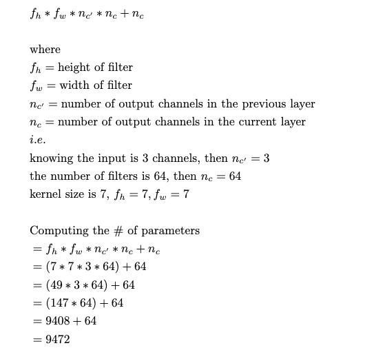
Let's understand this further from the layout. We have 64 filters in the convolution layer. Each filter is composed of three kernels, and each filter has a bias. So, if each kernel is 7 by 7, the number of parameters in each filter is 7 x 7 x 3 = 147 parameters. Given that we have 64 filters, then the weights across all the filters would be 147 by 64 which is 9408 parameters. And knowing that each filter has a bias, then add 64 parameters to the 9408 to get 9472 parameters.
Note: One interesting thing is that convolutional layers in ResNets do not have biases as they are in the Batch Normalization layers that follow, as said by Kaiming He. Let's understand why. Biases shift the weights in the parametrized layers as a whole to better optimize the curve. Batch Normalization in itself also does shift the activation by their mean values, hence serving the purpose of the bias in the convolution layers. Implementing bias in both convolution and Batch Normalization layers that follow each other is therefore redundant. When convolution layers in ResNets are therefore implemented, the biases are set to zero.

~remember to check if I've done this in the coming sections on implementing the residual block.

~ Number of parameters in linear layer.
Let's say we have 2048 inputs to a linear layer of 1000 neurons. We can that each neuron, from our very early section, is a perceptron with raw logits or an activation layer, but that apart, each has a bias. So the resulting number of parameters is 2,048,000 weights and 1,000 bias which is 2,049,000 parameters.

~ A nice short example
Let's create a linear topology of directed acrylic graph composed of three linear layers, assuming the input to be MNIST flattened image, that is 784 vector normalized values, and the output is 10 raw logits that are one softmax call away from being a probabilistic ditribution of the most likely digit of the image passed in.

import torch.nn as nn
model = nn.Sequential(
    nn.Linear(784, 392),
    nn.Linear(392, 196),
    nn.Linear(196, 10)
)

From the above code, the input is 784 features of a flattened image which first goes to the first hidden layer. This layer has 392 neurons. The output which for now has not been passed into activation layer to introduce non-linearity is then passed to the second hidden layer.
Hence, the input to the second hidden layer is 392, the output is 196. The output again, is then passed as an input to a third layer which then has 10 neurons. So the output of this third layer is 10 neurons. So, computing the parameters, we have:
For the first layer ~ 784 x 392 + 392
For the second layer ~ 392 x 196 + 196
For the third layer ~ 196 x 10 + 10
gives us the total of
307,720 + 77,028 + 1,970 = 386,718

import torch.nn as nn
model = nn.Sequential(
    nn.Linear(784, 392),
    nn.Linear(392, 196),
    nn.Linear(196, 10)
)

            >>> total_parameters = sum([p.numel() for p in model.parameters()])
>>> print(total_parameters)
386718
          

Unpausing the time

Now that we have gone back to understanding every single detail needed to implement a residual block (and the whole ResNet or so it seems), let's start off the next section with implementing it.