66 years too soon

The year is July 1958, the unveiling is by the Office of Naval Research, the creator, Frank Rosenblatt, the invention, perceptron. So what is it?

“the first machine capable of having an original idea” ~ Frank Rosenblatt

This invention was first inspired by the working of neurons in the brain, and so it was of concern to build a machine that could classify a given input into two categories, let's say a cat or a dog - and if wrong, would then tweak itself to make a more informed prediction the next time.
Rosenblatt wrote ~ “Yet we are about to witness the birth of such a machine – a machine capable of perceiving, recognizing and identifying its surroundings without any human training or control.”
Marvin Minsky, a fellow, however commented that the functions were just too simple hence perceptron could never achieve its goal.

And I quote this article from Cornell

Professor’s perceptron paved the way for AI – 60 years too soon

The problem was, Rosenblatt’s perceptron had only one layer, while modern neural networks have millions.

“What Rosenblatt wanted was to show the machine objects and have it recognize those objects. And 60 years later, that’s what we’re finally able to do,” Joachims said. “So he was heading on the right track, he just needed to do it a million times over. At the time, he didn’t know how to train networks with multiple layers. But in hindsight, his algorithm is still fundamental to how we’re training deep networks today.”

Onto the classical model of a perceptron, the first ever linear classifier
Mark Hasegawa-Johnson, CS 440, Spring 2018

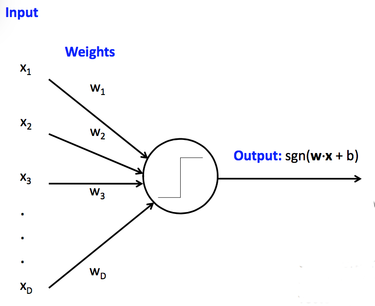
What essentially happens in a perceptron? There's inputs, a vector x, and the weights, a vector, w, and a scalar value, a bias. The operations are a dot product of x and w to get an output which is then added to the bias. This is then passed to the signum function to obtain the final output of the perceptron.
Note: The first perceptron ever implemented was a machine, rather than a program. It was implemented in a custom built hardware, "Mark-1 perceptron", and was purely an analog computer with knobs to adjust the weights and weight updates during learning performed by electric motors.
Originally, the perceptron used a step function. For the one in the figure, a signum function is used.
Let's implement it using Pytorch.

class Perceptron:
    """
    for now, i'll not use the computational graph 
    just for understanding of the learning of the 
    perceptron i.e. 
    I'll not declare a graph tracked
    computation using require_grads=True
    """
    def __init__(self, shape_x):
        super().__init__()
        self.w = torch.randn(shape_x)
        self.b = torch.randn(1)
        
    def __call__(self, x):
        out = torch.dot(x, self.w) + self.b
        yhat = torch.sign(out)
        return yhat
    
x = torch.tensor([1., 1.])
print(x.shape)
perceptron = Perceptron(x.shape)
print(perceptron(x))

            torch.Size([2])
tensor([-1.])
          

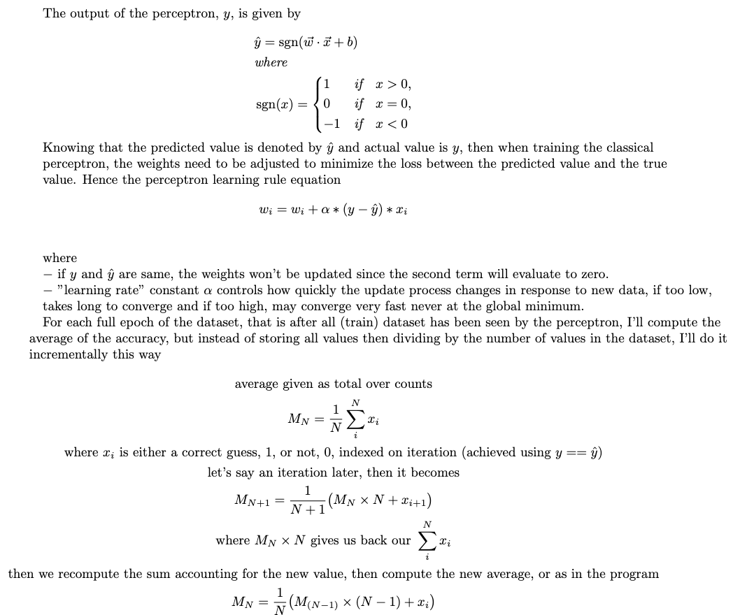
An input will be passed to the perceptron, to compute dot product and pass through the activation function sgn to get output yhat, in the forward pass. This will be used together with actual value y in the loss function, in our case a simple y-yhat, which will then guide the adjustments for the weights during the perceptron learning rule, discussed next.
This, for a general complex neural network, is going back the computational graph computing the gradients till the leaf Tensors then using the .grad values of each node in the network to compute the new weights in the network in hopes of convergence to the minimum in the backward pass. Then repeating again!
Now onto the perceptron learning rule, in the modern day it is known as updating the weights using optimizers such as Stochastic Gradient Descent or Adam in the backward pass.

torch.manual_seed(42)

class Perceptron:
    def __init__(self, shape_x):
        super().__init__()
        self.w = torch.randn(shape_x)
        self.b = torch.randn(1)
        self.count = 1
        self.avg = 0
        self.avgs = []
        
    def __call__(self, x, y, i, N, alpha = 0.001):
        out = torch.dot(x, self.w) + self.b
        yhat = torch.sign(out)
        # update 
        if yhat != y:
            self.w = self.w + alpha * (y - yhat) * x
            self.b = self.b + alpha * (y - yhat)
        # score
        self.avg = (self.avg * (self.count - 1) + (yhat == y)) / self.count
        self.count += 1
        # reset scores
        if i == 0:
            self.avg = 0
            self.count = 1
        elif i == N - 1:
            avg = self.avg.numpy()[0]
            self.avgs.append(avg)
            print(f"accuracy: {avg:.2f}")
        # return prediction
        return yhat

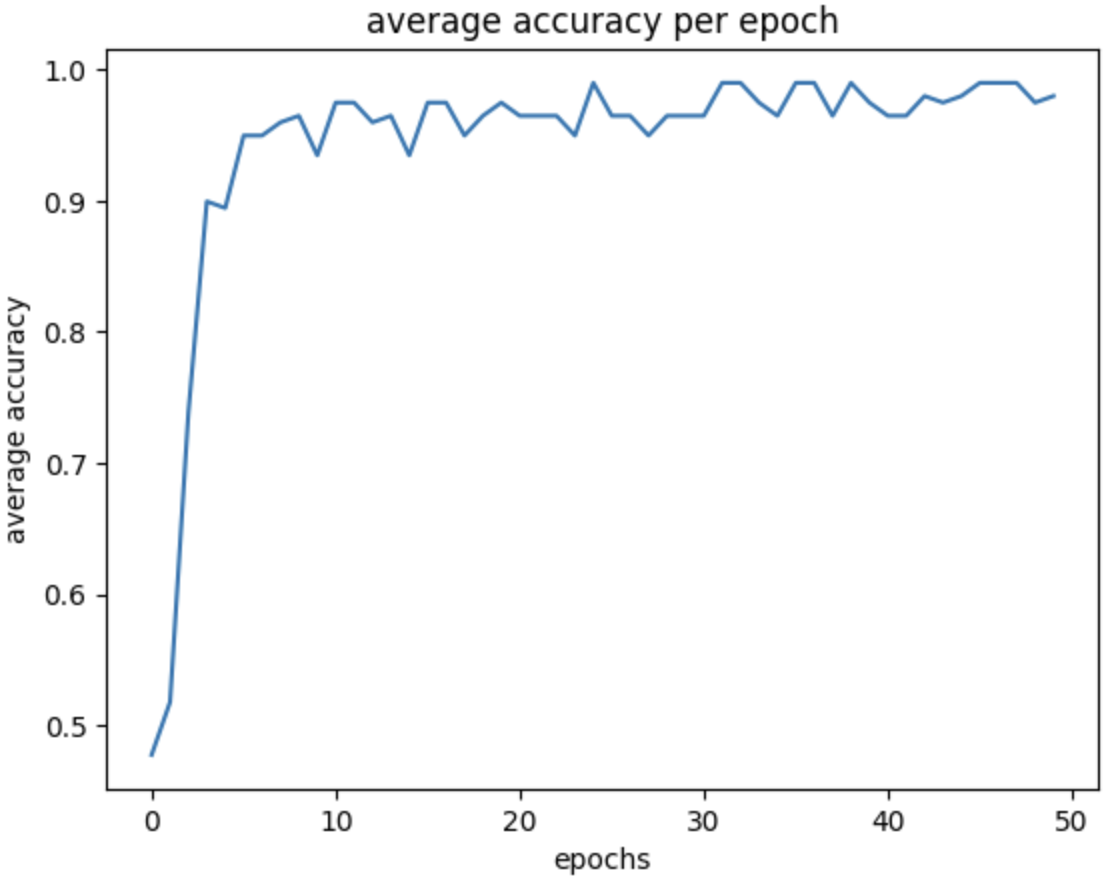
Now, let's make a small change to our class above, add method called predict for predicting new values once we have trained our perceptron model, and plot, for visualizing the average accuracy for each epoch all the way to the last epoch, no early stopping mechanism implemented.

import matplotlib.pyplot as plt
torch.manual_seed(42)

class Perceptron:
    def __init__(self, shape_x):
        super().__init__()
        self.w = torch.randn(shape_x)
        self.b = torch.randn(1)
        self.count = 1
        self.avg = 0
        self.avgs = []
        
    def __call__(self, x, y, i, N, alpha = 0.001):
        out = torch.dot(x, self.w) + self.b
        yhat = torch.sign(out)
        # update 
        self.w = self.w + alpha * (y - yhat) * x
        self.b = self.b + alpha * (y - yhat)
        # score
        self.avg = (self.avg * (self.count - 1) + (yhat == y)) / self.count
        self.count += 1
        if i == 0:
            self.avg = 0
            self.count = 1
        elif i == N - 1:
            avg = self.avg.numpy()[0]
            self.avgs.append(avg)
            print(f"accuracy: {avg:.2f}")
        return yhat

    def predict(self, x):
        out = torch.dot(x, self.w) + self.b
        yhat = torch.sign(out)
        return yhat
        
    def plot(self):
        plt.title("average accuracy per epoch")
        plt.xlabel("epochs")
        plt.ylabel("average accuracy")
        plt.plot(self.avgs)

linearly separable data

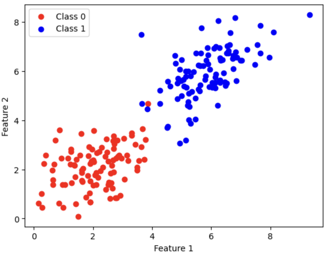
Now that we have implemented our perceptron, let us create data to train it on. Since perceptron is a linear classifier, it can only learn linearly separable functions, that is, the two sets in the data due to mapping by the function can be separated by at least one line in the plane. The code below does generate the data for us. Because it is not the focus of the course, I will not explain it, also it is not hard to understand.

# for reproducibility on rerunning the code
np.random.seed(42)

# 100 of each class created
# 200 samples of train data (total) created
N = 100

classes = [
    {"mean": [2, 2],
     "cov": [[1, 0.5], [0.5, 1]]},
    {"mean": [6, 6],
     "cov": [[1, 0.5], [0.5, 1]]}
]

# linearly separable data
X = np.vstack([np.random.multivariate_normal(c["mean"], c["cov"], N) for c in classes])
y = np.hstack((np.full(N, -1), np.ones(N))) # two distinct outputs, aligning with sgn output

# shuffling the data, a necessary step to avoid model
# bias in general neural networks
p = np.random.permutation(X.shape[0])
X, y = X[p], y[p]

On visualizing the dataset, except for a single sample which we can consider an outlier, we can draw a single line to distinguish the two classes

plt.scatter(X[y == -1][:, 0], X[y == -1][:, 1], color='red', label='Class 0')
plt.scatter(X[y == 1][:, 0], X[y == 1][:, 1], color='blue', label='Class 1')
plt.xlabel('Feature 1')
plt.ylabel('Feature 2')
plt.legend()
plt.show()

Nice! Now, let's see the performance of our perceptron right before we train it to see how badly it is with the randomly initialized weights.

accuracy = 0
count = 1

for _x, _y in zip(X, y):
    pred = perceptron.predict(torch.tensor(_x, dtype=torch.float32))
    pred = pred.numpy()[0]
    accuracy = (accuracy * (count - 1) + (pred == _y)) / count
    count += 1    
print(f"accuracy: {accuracy:.2f}")
# accuracy: 0.50

Accuracy is at 50%, meaning it performs as good as a fair coin toss experiment. Now let's train the perceptron.

perceptron = Perceptron(X[0].shape)

t = 10_000
N = X.shape[0]

for i in range(t):
    x = torch.Tensor(X[i % N])
    actual = y[i % N] 
    pred = perceptron(x, actual, i % N, N)
perceptron.plot()

            accuracy: 0.48
accuracy: 0.52
accuracy: 0.74
accuracy: 0.90
accuracy: 0.89
accuracy: 0.95
accuracy: 0.95
accuracy: 0.96
accuracy: 0.96
accuracy: 0.93
accuracy: 0.97
accuracy: 0.97
accuracy: 0.96
accuracy: 0.96
accuracy: 0.93
accuracy: 0.97
accuracy: 0.97
accuracy: 0.95
accuracy: 0.96
accuracy: 0.97
accuracy: 0.96
accuracy: 0.96
accuracy: 0.96
accuracy: 0.95
accuracy: 0.99
accuracy: 0.96
accuracy: 0.96
accuracy: 0.95
accuracy: 0.96
accuracy: 0.96
accuracy: 0.96
accuracy: 0.99
accuracy: 0.99
accuracy: 0.97
accuracy: 0.96
accuracy: 0.99
accuracy: 0.99
accuracy: 0.96
accuracy: 0.99
accuracy: 0.97
accuracy: 0.96
accuracy: 0.96
accuracy: 0.98
accuracy: 0.97
accuracy: 0.98
accuracy: 0.99
accuracy: 0.99
accuracy: 0.99
accuracy: 0.97
accuracy: 0.98
          

Now on running this again

accuracy = 0
count = 1

for _x, _y in zip(X, y):
    pred = perceptron.predict(torch.tensor(_x, dtype=torch.float32))
    pred = pred.numpy()[0]
    accuracy = (accuracy * (count - 1) + (pred == _y)) / count
    count += 1    
print(f"accuracy: {accuracy:.2f}")

            accuracy: 0.98
          

And that would be a wrap for awesome learning of perceptron algorithm.